Hi sm.hasehmin,

You can use the Bioconductor package karyoploteR for this. You can plot the data as points using kpPoints as in the example below or you could change that to kpSegments to show the width of your data elements, for example. There's more information on the available functions and customization options at the karyoploteR tutorial.

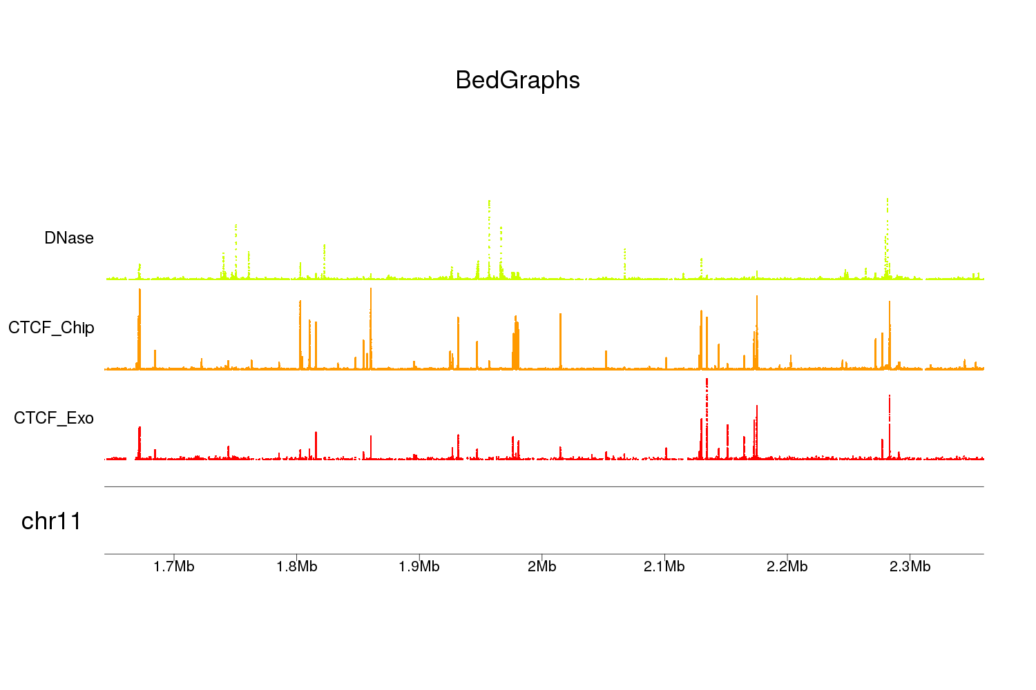
To load the bedgraphs into R you can use toGRanges from regioneR. In the example I'm using bedgraph example data from Sushi which is not CNV data, but with only minor changes (setting ymin and ymax) you should be able to adapt the code to CNV values. To load your data, you can give toGRanges the file name of your bedgraphs and it should load them.

For the vertical positioning (r0 and r1) I'm using autotrack. This function is not yet in the tutorial but the inline documentation should suffice.

Note: since the example datasets have only data for a small region of chromosome 11 this is what we are plotting. Removing the zoom argument from plotKaryotype will plot the whole genome.

#Load 3 example bedgraphs from the datasets in the Sushi package
library(Sushi)
data(list=c("Sushi_DNaseI.bedgraph","Sushi_ChIPSeq_CTCF.bedgraph",
        "Sushi_ChIPExo_CTCF.bedgraph"), package="Sushi")

dd <- list(CTCF_Exo=Sushi_ChIPExo_CTCF.bedgraph,
           CTCF_Chip=Sushi_ChIPSeq_CTCF.bedgraph,
           DNase=Sushi_DNaseI.bedgraph)

png("bedgraphPlot.png", width = 1500, height = 1000)
  kp <- plotKaryotype(zoom="chr11:1643216-2359707", main = "BedGraphs", cex=3)
  kpAddBaseNumbers(kp, tick.dist = 10e4, add.units = TRUE, cex=1.8)
  for(i in seq_len(length(dd))) {
    names(dd[[i]]) <- c("chr", "start", "end", "value") 
    gr <- toGRanges(dd[[i]])
    at <- autotrack(i, length(dd), margin = 0.1)
    kpPoints(kp, data=gr, ymax=max(gr$value), r0=at$r0, r1=at$r1, col=rainbow(10)[i])
    kpAddLabels(kp, labels = names(dd)[i], r0=at$r0, r1=at$r1, cex=2)
  }
dev.off()

And you would get something like this