
The code and approaches that I share here are those I am using to analyze TCGA methylation data. At the bottom of the page, you can find references used to make this tutorial. If you are coming from a computer background, please bear with a geneticist who tried to code :). Your feedback is worth a lot to me.
The three main analyses of methylation data are covered:
1- differential methylation analysis
2- differential variability analysis
3- integrative analysis
For code and files, you can check my GitHub. For this post, I used publicly available data from TCGA bladder cancer (TCGA-BLCA) for methylation and gene expression analysis.
Workspace preparation
#______________loading packages__________________#
library(TCGAbiolinks)
library(IlluminaHumanMethylation450kanno.ilmn12.hg19)
library(IlluminaHumanMethylation450kmanifest)
library(minfi)
library(limma)
library(missMethyl)
library(DMRcate)
library(Gviz)
library(ggplot2)
library(RColorBrewer)
library(edgeR)

#increase memory size
memory.limit(size = 28000) # do this on your own risk!
Data download and preparation
#_________ DNA methylation Download____________#
# DNA methylation aligned to hg19
query_met <- GDCquery(project= "TCGA-BLCA",
                           data.category = "DNA methylation",
                           platform = "Illumina Human Methylation 450",
                           legacy = TRUE)
GDCdownload(query_met)
#putting files together
data.met <- GDCprepare(query_met)
#saving the met object
saveRDS(object = data.met,
        file = "data.met.RDS",
        compress = FALSE)
# loading saved session: Once you saved your data, you can load it into your environment:
data.met = readRDS(file = "data.met.RDS")
# met matrix
met <- as.data.frame(SummarizedExperiment::assay(data.met))
# clinical data
clinical <- data.frame(data.met@colData)

#___________inspecting methylation data_______________#

# get the 450k annotation data
ann450k <- getAnnotation(IlluminaHumanMethylation450kanno.ilmn12.hg19)

## remove probes with NA
probe.na <- rowSums(is.na(met))

table(probe.na == 0)
#FALSE   TRUE
#103553 382024
# chose those has no NA values in rows
probe <- probe.na[probe.na == 0]
met <- met[row.names(met) %in% names(probe), ]

## remove probes that match chromosomes X and Y
keep <- !(row.names(met) %in% ann450k$Name[ann450k$chr %in% c("chrX","chrY")])
table(keep)
met <- met[keep, ]
rm(keep) # remove no further needed probes.

## remove SNPs overlapped probe
table (is.na(ann450k$Probe_rs))
# probes without snp
no.snp.probe <- ann450k$Name[is.na(ann450k$Probe_rs)]

snp.probe <- ann450k[!is.na(ann450k$Probe_rs), ]
#snps with maf <= 0.05
snp5.probe <- snp.probe$Name[snp.probe$Probe_maf <= 0.05]

# filter met
met <- met[row.names(met) %in% c(no.snp.probe, snp5.probe), ]

#remove no-further needed dataset
rm(no.snp.probe, probe, probe.na, snp.probe, snp5.probe)

## Removing probes that have been demonstrated to map to multiple places in the genome.
# list adapted from https://www.tandfonline.com/doi/full/10.4161/epi.23470

crs.reac <- read.csv("cross_reactive_probe.chen2013.csv")
crs.reac <- crs.reac$TargetID[-1]

# filtre met
met <- met[ -which(row.names(met) %in% crs.reac), ]
bval <- met

## converting beta values to m_values
## m = log2(beta/1-beta)
mval <- t(apply(met, 1, function(x) log2(x/(1-x))))
#______________saving/loading_____________________#
# save data sets
#saveRDS(mval, file = "mval.RDS", compress = FALSE)
#saveRDS (bval, file = "bval.RDS", compress = FALSE)
#mval <- readRDS("mval.RDS")
#bval <- readRDS("bval.RDS")
Differential methylation analysis
Different methylated CpGs (DMC) or Probe-wise differential methylation analysis
Here we are interested to find probes that are differentially methylated between low-grade and high-grade bladder cancer. In the clinical dataset, there is column paper_Histologic.grade that provides data on tumor grade. Also as one can see, most low-grade bladder cancer samples belong to the luminal papillary subtype.
I have to make it clear that for assigning "low-grade" or "high-grade" to a sample I relied on the clinical data published by A Gordon Robertson, however, it is acknowledged that those samples in the Ta stage should be considered as "low-grade", samples with T1 and upper stages are "high-grade". By the way, this would not affect a bioinformatic analysis!
table(clinical$paper_Histologic.grade, clinical$paper_mRNA.cluster)
# Basal_squamous Luminal Luminal_infiltrated Luminal_papillary ND Neuronal
# High Grade 143 28 79 120 4 20
# Low Grade 1 0 0 20 0 0
# ND 0 0 1 2 0 0
# filtering and grouping
clinical <- clinical[, c("barcode", "paper_Histologic.grade", "paper_mRNA.cluster")]
clinical <- na.omit(clinical)
clinical <- clinical[-which(clinical$paper_mRNA.cluster == "ND"), ]
clinical <- clinical[-which(clinical$paper_Histologic.grade == "ND"), ]
clinical <- clinical[which(clinical$paper_mRNA.cluster == "Luminal_papillary"), ]
barcode <- clinical$barcode
# removing samples from meth matrixes
bval <- bval[, colnames(bval) %in% barcode]
mval <- mval[, colnames(mval) %in% barcode]
# Making sure about samples in clinical and matrixes and their order
table(colnames(mval) %in% row.names(clinical))
table(colnames(bval) %in% row.names(clinical))
#
all(row.names(clinical) == colnames(bval))
all(row.names(clinical) == colnames(mval))
#Making grouping variable
clinical$paper_Histologic.grade <- as.factor(clinical$paper_Histologic.grade)
#levels(clinical$paper_Histologic.grade)
clinical$paper_Histologic.grade <- relevel(clinical$paper_Histologic.grade, ref = "Low Grade")
#_____________ DMC analysis________________#
design <- model.matrix(~ paper_Histologic.grade, data = clinical)
# fit the linear model
fit <- lmFit(mval, design)
fit2 <- eBayes(fit)
# extracting significantly methylated probes
deff.meth = topTable(fit2, coef=ncol(design), sort.by="p",number = nrow(mval), adjust.method = "BY")
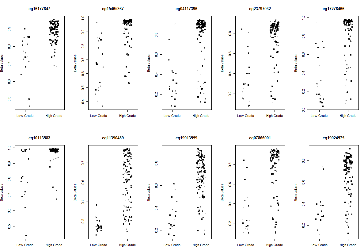
# Visualization
# plot the top 10 most significantly differentially methylated CpGs
par(mfrow=c(2,5))
sapply(rownames(deff.meth)[1:10], function(cpg){
plotCpg(bval, cpg=cpg, pheno=clinical$paper_Histologic.grade, ylab = "Beta values")
})
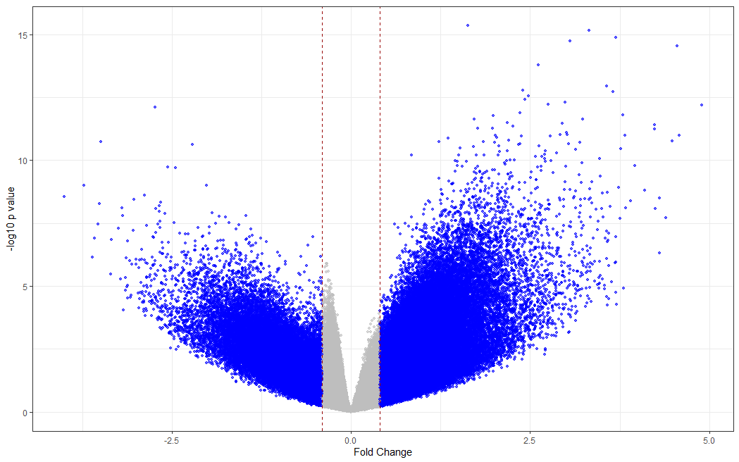
# making a volcano plot
#making dataset
dat <- data.frame(foldchange = fit[["coefficients"]][,2], logPvalue =  -log10(fit2[["p.value"]][,2]))
dat$threshold <- as.factor(abs(dat$foldchange) < 0.4)

#Visualization
cols <- c("TRUE" = "grey", "FALSE" = "blue")
ggplot(data=dat, aes(x=foldchange, y = logPvalue, color=threshold)) +
  geom_point(alpha=.6, size=1.2) +
  scale_colour_manual(values = cols) +
  geom_vline(xintercept = 0.4, colour="#990000", linetype="dashed") +
  geom_vline(xintercept = - 0.4, colour="#990000", linetype="dashed") +
  theme(legend.position="none") +
  xlab("Fold Change") +
  ylab("-log10 p value") +
  theme_bw() +
  theme(legend.position = "none")
Differentially methylated regions (DMRs) analysis
# setting some annotation
myAnnotation <- cpg.annotate(object = mval, datatype = "array",
what = "M",
analysis.type = "differential",
design = design,
contrasts = FALSE,
coef = "paper_Histologic.gradeHigh Grade",
arraytype = "450K",
fdr = 0.001)
str(myAnnotation)
# DMR analysis
DMRs <- dmrcate(myAnnotation, lambda=1000, C=2)
results.ranges <- extractRanges(DMRs)
results.ranges
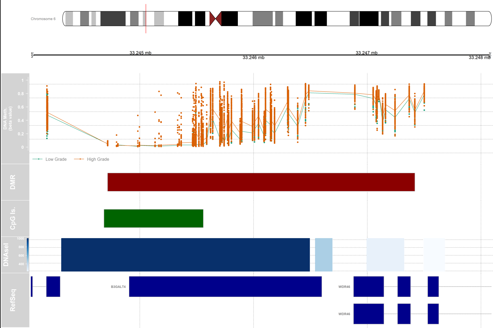
# visualization
dmr.table <- data.frame(results.ranges)
# setting up a variable for grouping and color
pal <- brewer.pal(8,"Dark2")
groups <- pal[1:length(unique(clinical$paper_Histologic.grade))]
names(groups) <- levels(factor(clinical$paper_Histologic.grade))
#setting up the genomic region
gen <- "hg19"
# the index of the DMR that we will plot
dmrIndex <- 2
# coordinates are stored under results.ranges[dmrIndex]
chrom <- as.character(seqnames(results.ranges[dmrIndex]))
start <- as.numeric(start(results.ranges[dmrIndex]))
end <- as.numeric(end(results.ranges[dmrIndex]))
# add 25% extra space to plot
minbase <- start - (0.25*(end-start))
maxbase <- end + (0.25*(end-start))
# defining CpG islands track
# download cpgislands for chromosome number 6 from ucsc
chr6.cpg <- read.csv("chr6-cpg.csv")
islandData <- GRanges(seqnames=Rle(chr6.cpg[,1]),
ranges=IRanges(start=chr6.cpg[,2],
end=chr6.cpg[,3]),
strand=Rle(strand(rep("*",nrow(chr6.cpg)))))
# DNAseI hypersensitive sites track
#downloaded from ucsc
chr6.dnase <- read.csv("chr6-dnase.csv")
dnaseData <- GRanges(seqnames=chr6.dnase[,1],
ranges=IRanges(start=chr6.dnase[,2], end=chr6.dnase[,3]),
strand=Rle(rep("*",nrow(chr6.dnase))),
data=chr6.dnase[,5])
#Setting up the ideogram, genome, and RefSeq tracks
iTrack <- IdeogramTrack(genome = gen, chromosome = chrom, name=paste0(chrom))
gTrack <- GenomeAxisTrack(col="black", cex=1, name="", fontcolor="black")
rTrack <- UcscTrack(genome=gen, chromosome=chrom, track="NCBI RefSeq",
from=minbase, to=maxbase, trackType="GeneRegionTrack",
rstarts="exonStarts", rends="exonEnds", gene="name",
symbol="name2", transcript="name", strand="strand",
fill="darkblue",stacking="squish", name="RefSeq",
showId=TRUE, geneSymbol=TRUE)
#Ensure that the methylation data is ordered by chromosome and base position.
ann450kOrd <- ann450k[order(ann450k$chr,ann450k$pos),]
bvalOrd <- bval[match(ann450kOrd$Name,rownames(bval)),]
#Create the data tracks:
# create genomic ranges object from methylation data
cpgData <- GRanges(seqnames=Rle(ann450kOrd$chr),
ranges=IRanges(start=ann450kOrd$pos, end=ann450kOrd$pos),
strand=Rle(rep("*",nrow(ann450kOrd))),
betas=bvalOrd)
# methylation data track
methTrack <- DataTrack(range=cpgData,
groups=clinical$paper_Histologic.grade, # change this if your groups are different
genome = gen,
chromosome=chrom,
ylim=c(-0.05,1.05),
col=pal,
type=c("a","p"),
name="DNA Meth.\n(beta value)",
background.panel="white",
legend=TRUE,
cex.title=0.8,
cex.axis=0.8,
cex.legend=0.8)
# CpG island track
islandTrack <- AnnotationTrack(range=islandData, genome=gen, name="CpG Is.",
chromosome=chrom,fill="darkgreen")
# DNaseI hypersensitive site data track
dnaseTrack <- DataTrack(range=dnaseData, genome=gen, name="DNAseI",
type="gradient", chromosome=chrom)
# DMR position data track
dmrTrack <- AnnotationTrack(start=start, end=end, genome=gen, name="DMR",
chromosome=chrom,fill="darkred")
# Set up the tracklist and indicate the relative sizes of the different tracks.
# Finally, draw the plot using the plotTracks function
tracks <- list(iTrack, gTrack, methTrack, dmrTrack, islandTrack, dnaseTrack,
rTrack)
sizes <- c(2,2,5,2,2,2,3) # set up the relative sizes of the tracks
# to save figure and scaling graphic device
tiff( filename = "dmr.tiff", width = 15, height = 10, units = "in", res = 400)
plotTracks(tracks, from=minbase, to=maxbase, showTitle=TRUE, add53=TRUE,
add35=TRUE, grid=TRUE, lty.grid=3, sizes = sizes, length(tracks))
dev.off()
References
thank you so much it was really useful to me
Thank you very much for this useful tutorial. I was just wondering how one could annotate data for hg38 when legacy = FALSE?
This will return data for hg38 while legacy = FALSE:
the hg38 aligned methylation data doesn't return any result for TCGA AML working for hg19 only
Greetings dear Hamid Ghaedi Thanks for your nice and clear tutorial. Can you kindly share "cross_reactive_probe.chen2013.csv" file? I have been searching to find it publicly, but unfortunately didn't find it. Thanks in advance. Javad Karimbayli
File is available on GitHub site linked in original post: https://github.com/hamidghaedi/Methylation_Analysis/blob/master/cross_reactive_probe.chen2013.csv
Wondering if cross-reactive probes list is also available for EPIC array as well .. https://www.tandfonline.com/doi/full/10.4161/epi.23470
I think I found it here https://github.com/sirselim/illumina450k_filtering . however final list has 135885 unique probes to remove, which seems to be very high.
Thank you so much for this guide. I have just few problems to plot the DMR with both this method and dmr plot function. The error is related to a specific cookie called Hguid. I tried to make the plot track separated like this with downloaded local info but i'm not able to plot the dmr again. How can I solve this problem? Thanks in advance
Could you show what you have tried and post the error that you have got?
Hello professor! Thank you very much for the detailed analysis!! I have some questions on the track plot;
1) Do the subsequent tracks concern only the area of the chromosome that has been highlighted by the small red vertical bar?
2) What does the length of each bar show (for the DMR and CpG for example) ?
Thank you in advance!!
Best regards,
Kostas.
Hi Kostas, thanks for showing interest on this post.
Yes
The length of bars in each track corresponds to the distance between the start and end of that element on the chromosomal coordinate. In the case of DMR, the bar size corresponds to the length of the differentially methylated region. In the case of CpG islands, the length is proportional to the length of the CpG island present in that location of the genome.
Hello once again!
Thank you very much for answering my questions!! Your feedback is very helpful!!!
Pardon my ignorance but I have one more question regarding controlStripPlots; So far I have understood that it is a way of performing quality control on methylation array data. Each row represents a sample and each column is a beta intensity value (logarithmized) and this is done for both channels (red and green).
What has got me a bit confused is the interpretation of the results that we get.
The way I have understood it, is that for instance, if we want to check the Bisulfite Conversion control probes, we essentially get a glimpse of how well bisulfite sequencing has been performed (methylated Cytosines left as is and unmethylated one replaced by Uracil and subsequently by Thymine). So, considering that bisulfite sequencing performs that conversion, does that mean that we expect that the values of the red channel will be a bit higher compared to the green channel? Is that a correct way to interpret the plot (in the context of bisulfite sequencing at least) ? Is there something else that I'm missing or that I have completely confused?
Again, thank you very much for your valuable feedback!
Update; I think I have found the answer to my question in the official documentation for illumina's control probes here
Best regards, Kostas.