Credits to Tiago Silva; https://f1000research.com/articles/5-1542
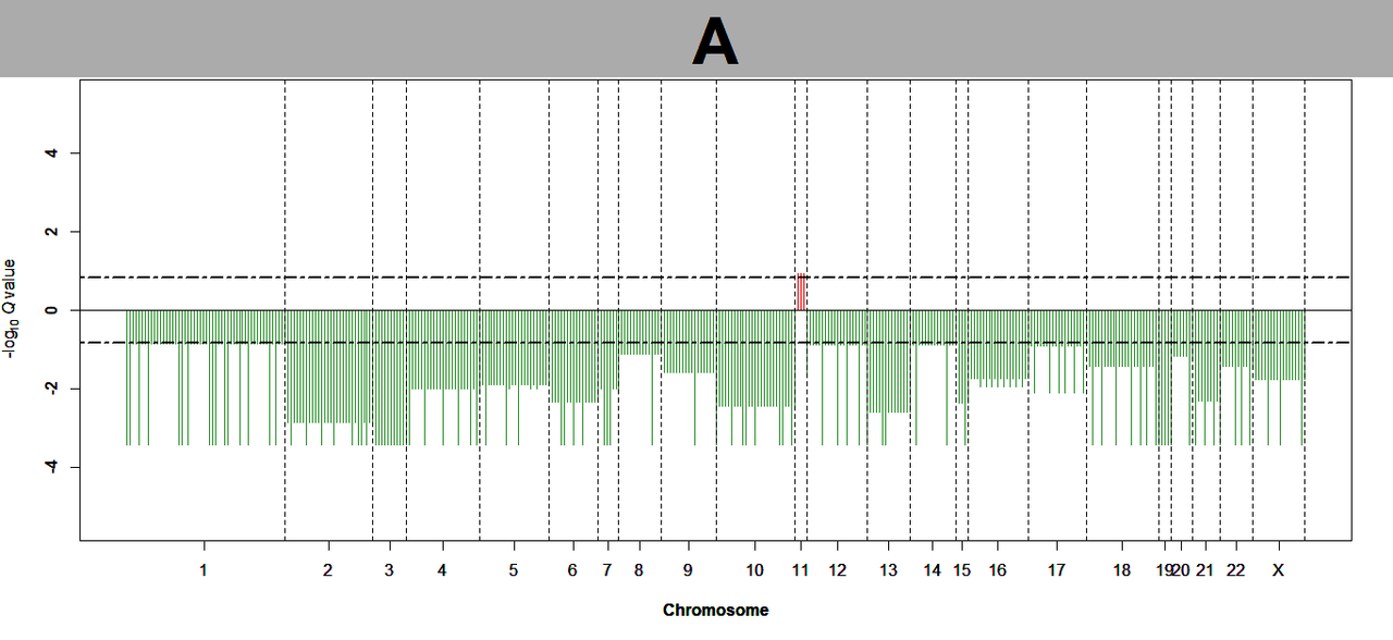
Ignording VEP, with output from runGAIA(), which identifies recurrent somatic copy number alterations (sCNAs), you can generate a plot like this:
Part I - download segmented sCNA data for any TCGA cohort from Broad Institute's FireBrowse server and identify recurrent sCNA regions in these with GAIA
Part II - plot recurrent sCNA gains and losses from GAIA
Part III - annotate the recurrent sCNA regions (this post, just below)
- Part IV -
generate heatmap of recurrent sCNA regions over your cohort
Part II
run runGAIA
results <- runGAIA(cnv_obj, markers_obj, output_file_name="Tumor.asian.txt", aberrations=-1, chromosomes=-1, num_iterations=10, threshold=0.15)
tidy output
#Set qvalue threshold for plotting and annotation
threshold <- 0.15

#Convert the recurrent aberrations to numeric (GAIA saves it as text)
RecCNV <- t(apply(results, 1, as.numeric))
colnames(RecCNV) <- colnames(results)

#Add a new column for 'score'
RecCNV <- cbind(RecCNV, score=0)

#Determine the minimum Q value that's not equal to 0
minval <- format(min(RecCNV[RecCNV[,"q-value"]!=0, "q-value"]), scientific=FALSE)
minval <- substring(minval,1, nchar(minval)-1)

#Replace Q values of 0 with the minimum, non-zero value
RecCNV[RecCNV[,"q-value"]==0, "q-value"] <- as.numeric(minval)

#Set the score to equal -log base 10 of the Q value
RecCNV[,"score"] <- sapply(RecCNV[,"q-value"], function(x) -log10(as.numeric(x)))
create plot function
#Create a function for plotting the recurrent copy number variants
gaiaCNVplot <- function (calls, threshold=0.01, main="main") {
    Calls <- calls[order(calls[,"Region Start [bp]"]),]
    Calls <- Calls[order(Calls[,"Chromosome"]),]
    rownames(Calls) <- NULL
    Chromo <- Calls[,"Chromosome"]
    Gains <- apply(Calls,1,function(x) ifelse(x["Aberration Kind"]==1, x["score"], 0))
    Losses <- apply(Calls, 1,function(x) ifelse(x["Aberration Kind"]==0, x["score"], 0))
    plot(Gains, ylim=c(-max(Calls [,"score"]+2), max(Calls[,"score"]+2)), type="h", col="red2", xlab="Chromosome", ylab=expression("-log"[10]~italic(Q)~"value"), main=main, cex.main=4, xaxt="n", font=2, font.axis=2, font.lab=2, font.axis=2)
    points(-(Losses), type="h", col="forestgreen")
    abline(h= 0, cex=4)
    abline(h=-log10(threshold), col="black", cex=4, main="test", lty=6, lwd=2)
    abline(h=log10(threshold), col="black", cex=4, main="test", lty=6, lwd=2)
    uni.chr <- unique(Chromo)
    temp <- rep(0, length(uni.chr))

    for (i in 1:length(uni.chr)) {
        temp[i] <- max(which(uni.chr[i] == Chromo))
    }

    for (i in 1:length(temp)) {
        abline(v = temp[i], col = "black", lty = "dashed", )
    }

    nChroms <- length(uni.chr)

    begin <- c()

    for (d in 1:nChroms) {
        chrom <- sum(Chromo == uni.chr[d])
        begin <- append(begin, chrom)
    }

    temp2 <- rep(0, nChroms)

    for (i in 1:nChroms) {
        if (i == 1) {
            temp2[1] <- (begin[1] * 0.5)
        }
        else if (i > 1) {
            temp2[i] <- temp[i - 1] + (begin[i] * 0.5)
        }
    }

    uni.chr[uni.chr==23] <- "X"
    uni.chr[uni.chr==24] <- "Y"

    for (i in 1:length(temp)) {
        axis(1, at = temp2[i], labels = uni.chr[i], cex.axis = 1)
    }

    #legend("topright", y.intersp=0.8, c("Amplification"), pch=15, col=c("red2"), text.font=2)
    #legend("bottomright", y.intersp=0.8, c("Deletion"), pch=15, col=c("forestgreen"), text.font=2)
}
plot data
gaiaCNVplot(RecCNV, threshold, "A")

Kevin
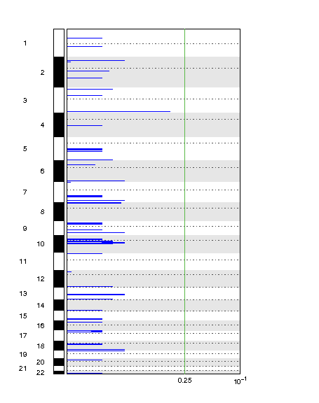


VEP and GISTIC are apple and orange, IMO. Not clear how the analysis is done. Did you try other CNA tools using CBS or Haar algorithms?
Do you have an example image for Deletion depiction?
This is the link: https://postimg.cc/yDv16Z8q
Nazanin, as I understood from the previous question, you only wanted to use VEP for the purpose of annotating the regions. VEP is usually the end-point in an analysis, i.e., the final step.
Going back to this step: C: Annotation of huge number of CNV files
Were you ever able to run that command (
runGAIA()) successfully? It will likely not work on any personal computer because it is too compute intensive.Again, the pipeline that works is this:
Yes Kevin, you're right.
If you remember after getting the result of copy number analysis I tried to run biomaRt as you suggested to me. However I could not run it properly so I decided to use VEP instead. I have access to server right now, however I am a little confused about how I can generate a custom CNV plot to represent in my paper.
I tried to re-perform the analysis using gistic 2.0 on Genepattern, however no significant results was generated. This made me more confused.
Can you possibly retry the annotation step with biomaRt? The exact steps are here: A: How to extract the list of genes from TCGA CNV data
The previous thread became too long...
Sure. I will rerun biomaRt on Monday and let you know at which step I got the error message. I think the source of problem is what I introduce to biomaRt as input.
Thank you again
I have also just posted an answer below, showing how you can plot output from runGAIA. Let me know if it works.
If you need me to process the data for you on my servers, then I will do that - no problem. Just point me to which Firebrowse data you are using. You can contact me in private, if you wish.
Sure Kevin.
I will inform you on Monday.
Hi cpad, the original thread had dragged on, here: C: Annotation of huge number of CNV files
See: How to add images to a Biostars post
Hi @Kevin Blighe I am getting a similar plot like this one, all commands seem to run without any errors, exactly same steps followed form part I, part II and part III. Could you help with it?
Thank you
Do not add answers unless you're answering the top level question. "I have this problem too" comments should be comment-replies on appropriate posts, not answers. I've moved your post to a comment for now, but please be more careful in the future.