Library complexity downsampling validation and samtools flagstat (ATAC-seq)

Question

[reskejak]

I have been trying to downsample my ATAC-seq libraries to normalize across all samples within my experimental design using ATACseqQC::readsDupFreq|estimateLibComplexity, which is based on the established preseqR::ds.mincount.bootstrap framework. After scaling all libraries to the same predicted complexity, I am now encountering some inconsistencies in the library statistics.

Basic experimental design is two experimental groups (treat vs. control) with two biological replicates in each group = 4 libraries.

My basic workflow is to trim and align (PE75, Bowtie2), then:

samples=("treat1 treat2 control1 control2")
for i in $samples; do
# sort by coordinates
samtools sort -T /tmp/${i}.sorted -o ${i}.sorted.bam ${i}.bam;
# remove mtDNA reads via Harvard ATACseq tool
samtools view -h ${i}.sorted.bam | \
    python removeChrom.py - - chrM | samtools view -b - > ${i}.noMT.bam;
# sort by coordinates
samtools sort -T /tmp/${i}.sorted.noMT -o ${i}.sorted.noMT.bam ${i}.noMT.bam;
# index bam after mtDNA removal
samtools index ${i}.sorted.noMT.bam;
done

Then I assess for library complexity with the *.sorted.noMT.bam files. Here is a summarized output for total library and approximate common denominator within the experiment:

# full library
sample         relative.size    values      reads
treat1         1                16233349    19698535
treat2         1                20637534    21479224
control1       1                20355060    22131151
control2       1                15925428    17488379

# scaled to normalize (predicted)
sample         relative.size    values      reads
treat1         0.98             15943266    19304564
treat2         0.77             15970045    16539002
control1       0.78             15981835    17262297
control2       1                15925428    17488379

... where relative.size is the relative library size that yields specified values (estimated library size) and reads (estimated reads to achieve that library size).

I then subsample the files via samtools view -h -b -s:

samtools view -h -b -s 0.98 treat1.sorted.noMT.bam > treat1.sub.sorted.noMT.bam
samtools view -h -b -s 0.77 treat2.sorted.noMT.bam > treat2.sub.sorted.noMT.bam
samtools view -h -b -s 0.78 control1.sorted.noMT.bam > control1.sub.sorted.noMT.bam
# leave sample control2 as is (lowest complexity sample)

... and reassess complexity on subsampled files:

sample         relative.size    values      reads
treat1.sub     1                15944465    19304847
treat2.sub     1                15962582    16540771
control1.sub   1                15985716    17264865
control2       1                15925428    17488379

Looks like it worked. Excellent!

I then remove PCR duplicates via Picard MarkDuplicates, name-sort reads, samtools fixmate to facilitate downstream conversion to BEDPE for MACS2 peak calling:

samples=("treat1.sub treat2.sub control1.sub control2")
for i in $samples; do
# remove duplicates
java -jar picard.jar MarkDuplicates \
    I=${i}.sorted.noMT.bam \
    O=${i}.noDups.noMT.bam \
    M=${i}_dups.txt \
    REMOVE_DUPLICATES=true;
# name-sort reads
samtools sort -n ${i}.noDups.noMT.bam ${i}.sorted.noDups.noMT;
# fix mates
samtools fixmate ${i}.sorted.noDups.noMT.bam ${i}.fixed.bam;
done

Lastly, one final coordinate sort and index of the BAMs for csaw:

for i in $samples; do
samtools sort -T /tmp/${i}.sorted.fixed -o ${i}.sorted.fixed.bam ${i}.fixed.bam;
samtools index ${i}.sorted.fixed.bam;
done

Later on, a discrepancy is observed when we assess library size in csaw:

sample         lib.size
treat1.sub     17203692
treat1.sub     16057876
control1.sub   19706273
control2       19832246

... which is a summarized output of counts$totals.

Does this indicate we did not successfully compensate for library complexities by subsampling? Why are the calculated inter-sample library sizes different after subsampling?

Using samtools flagstat, I have tried to investigate this further. Here is a breakdown for sample treat2:

*.bam     *.noMT.bam *.sub.noMT.bam  *.sub.noDups.noMT.bam  *.sub.fixed.bam 
82159808  82159808   63269230        59839102               59839102          total
0          0         0               0                      0                 secondary
0          0         0               0                      0                 supplementary
0          0         0               0                      0                 duplicates
80032898  70040719   53936734        50506606               50506606          mapped
82159808  82159808   63269230        59839102               59719666          paired in sequencing
41079904  41079904   31634615        29905399               29859833          read1
41079904  41079904   31634615        29933703               29859833          read2
79045966  69160532   53259798        49963952               49963952          properly paired
79362718  69417198   53457164        50146472               50146472          with itself and mate mapped
670180    623521     479570          360134                 360134            singletons
82172     72510      55718           53420                  53420             mate mapped diff chr
27719     27056      20902           20302                  20302             mate mapped diff chr (mapQ>=5)

... or partially presented as a graph:

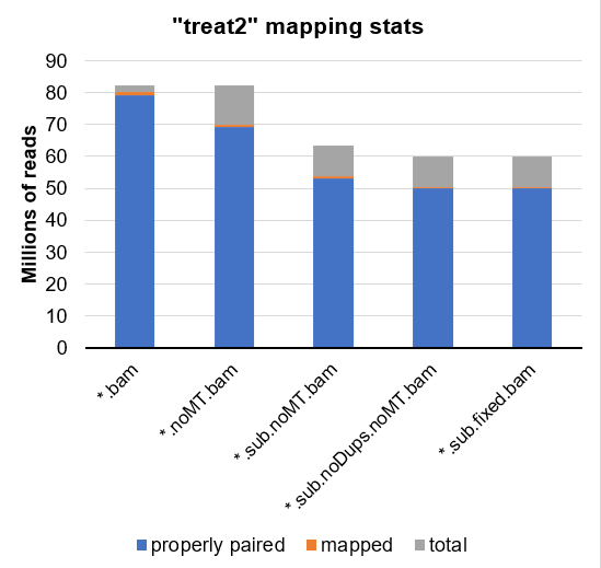
Could it be that the mtDNA are being read into csaw as true reads, even though they are not labeled as mapped?

Here is another look at all the final BAMs in this experiment which are subsequently loaded into csaw:

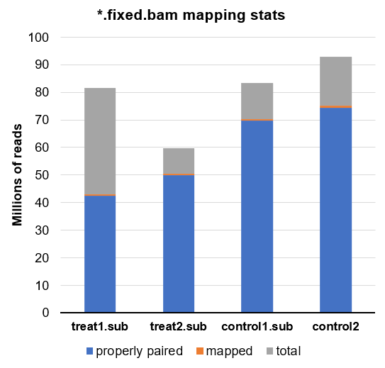
Comparing this to the library sizes calculated by csaw, we can tell even visually that the calculated sizes do not appear to match the read depth with or without mtDNA and whether or not it is utilized.

sample         lib.size
treat1.sub     17203692
treat1.sub     16057876
control1.sub   19706273
control2       19832246
# these are the same calculations from above

In conclusion, I do not understand why these libraries are showing highly variable read depths and library sizes when they should have been theoretically normalized to complexity. I am seeking explanation for this phenomenon and ultimately if I should trust 1) calculated library complexity estimates from preseqR/ATACseqQC or 2) csaw library size calculations. In the case of the latter, how can I correct my method?

Answer 1

[reskejak]

UPDATE:

Shortly after documenting all of this on paper, I realized I should be hard-filtering the mtDNA and unmapped reads from the libraries, as they may be still included in library size calculations even if they are not used. I revised my method to completely remove these reads and only retain the properly-paired read fragments (the bulk of the data) via samtools view -b -f 3 ${i}.sorted.noMT.bam > ${i}.filt.noMT.bam following the mtDNA removal step (which labels these reads as unmapped).

This worked wonderfully! After piping only the properly-paired reads (without mtDNA) into ATACseqQC for complexity estimates and subsequent normalization to these values, we later observe calculated library sizes in csaw as within 5% of the experimental mean, which I will accept as successfully normalized:

sample       lib.size
treat1       17661686
treat2       16429106
control1     17328942
control2     17324992

*small side note: I also pooled together some technical replicates to achieve slightly higher read depth, but same trends apply with original data set...

However, I have not been able to determine how the amount of unique reads scales with library complexity, as I was under the impression that they should be uniform. Strikingly, the BAM files used to elicit these results contain highly variable read counts from samtools flagstat:

sample        reads       fragments
treat1        43056518    21528259
treat2        50597792    25298896
control1      70049388    35024694
control2      74125640    37062820

This is essentially identical to the blue bars in the last plot of my original post. If we have removed all duplicates prior to generation of this BAM file, then how can we have highly variable read counts with the same library size and complexity?

Thanks in advance for any offered insight.

Edit: I think my understanding of library complexity may have been skewed; my understanding was that it refers to total number of molecules in a library, but it is also logical that it could refer to complexity of nucleotide sequences that compose the sequenced molecules (i.e. reads).

The latter idea would support my results: libraries which require more unique reads [than another sample to achieve a given complexity] would be composed of more simple repeats and low-complexity kmers. Can anyone confirm this rationale? Now excuse me while I go read through Daley and Smith's molecular complexity manuscript again more carefully...

Edit Edit: I determined the variable read counts in complexity-normalized libraries are to compensate for fragment size distributions. MACS2 calls predominant fragment length for these samples as 130, 119, 89, 85 respectively. Comparing these values to the read counts from samtools flagstat approximately line up: mean fragment length inversely correlates with read count. This logic is sound to me. Case closed!